Customer Segmentation Using Python In Machine Learning

MAIN PROJECT

Customer Segmentation is an unsupervised method of targeting the customers in order to increase sales and market goods in a better way

This project deals with real-time data where we have to segment the customers in the form f clusters using the K-Means algorithm

The data set consists of important variables like Age, Gender, annual income, etc.

With the help of the algorithms, we can easily visualize the data and can get a segmentation of each customer so that we can target the customers in the better way

Customer Segmentation is the subdivision of a market into discrete customer groups that share similar characteristics. Customer Segmentation can be a powerful means to identify unsatisfied customer needs. Using the above data companies can then outperform the competition by developing uniquely appealing products and services.

Advantages of Customer Segmentation

Determine appropriate product pricing.
Develop customized marketing campaigns.
Design an optimal distribution strategy.
Choose specific product features for deployment.
Prioritize new product development efforts.

Customer Segmentation using Python in Machine Learning Customer Segmentation is an unsupervised method of targeting the customers in order to increase sales and market goods in a better way

Installation and Software Requirements

In this project, we have used Anaconda which has various inbuilt software’s like Spyder, R, PyCharm, Jupyter, and much more

Utilizing Anaconda Environments in JupyterHub | Announce | University of Nebraska-Lincoln

For this specific project, we have used Jupyter notebook to run the codes

Anaconda is a distribution of the Python and R programming languages for scientific computing, that aims to simplify package management and deployment.

Language Used:

In this project, I have used python with machine learning

Python is an interpreted high-level general-purpose programming language.

Python is an interactive and object-oriented scripting language. Python is designed to be highly readable.

It supports functional and structured programming methods as well as OOP.

What is Python Coding? | Coding for Kids Ages 11+ | Juni Learning

It can be used as a scripting language or can be compiled to byte-code for building large applications.

It provides very high-level dynamic data types and supports dynamic type checking.

It supports automatic garbage collection.

Now let’s talk about Machine Learning !!

Machine Learning

Machine Learning is an application of Artificial Intelligence (AI) which enables a program(software) to learn from the experiences and improve itself at a task without being explicitly programmed. For example, how would you write a program that can identify fruits based on their various properties, such as color, shape, size, or any other

Machine Learning today has all the attention it needs. Machine Learning can automate many tasks, especially the ones that only humans can perform with their innate intelligence. Replicating this intelligence to machines can be achieved only with the help of machine learning.

Unsupervised Learning

Unsupervised learning is a machine learning technique in which models are not supervised using a training dataset. Instead, models themselves find the hidden patterns and insights from the given data. It can be compared to learning which takes place in the human brain while learning new things. Unsupervised learning cannot be directly applied to a

Entering the world of Machine Learning | by Ashley Sanders | Getting better, together. | Medium

regression or classification problem because, unlike supervised learning, we have the input data but no corresponding output data. The goal of unsupervised learning is to find the underlying structure of the dataset, group that data according to similarities, and represent that dataset in a compressed format.

K-Means Clustering

K-means clustering is a type of unsupervised learning, which is used when you have unlabeled data (i.e., data without defined categories or groups). The goal of this algorithm is to find groups in the data, with the number of groups represented by the variable K. The algorithm works iteratively to assign each data point to one of the K groups based on the features that are provided. Data points are clustered based on feature similarity.

Getting into the Project!

There are many libraries that go along with python few of them are Numpy, pandas,matplotlib In this project I have used few libraries in order to visualize the data in order to achieve better results.

Numpy

NumPy is the fundamental package for scientific computing in Python. It is a Python library that provides a multidimensional array object, various derived objects (such as masked arrays and matrices), and an assortment of routines for fast operations on arrays, including mathematical, logical, shape manipulation, sorting, selecting, I/O, discrete Fourier transforms basic linear algebra, basic statistical operations, random simulation and much more.

It is imported based on specific syntax like import numpy as np

Pandas

Pandas is a Python package that provides fast, flexible, and expressive data structures designed to make working with structured (tabular, multidimensional, potentially heterogeneous) and time-series data both easy and intuitive. It aims to be the fundamental high-level building block for doing practical, real-world data analysis in Python.

It is imported as import pandas as pd

Matplotlib

Matplotlib is an amazing visualization library in Python for 2D plots of arrays. Matplotlib is a multi-platform data visualization library built on NumPy arrays and designed to work with the broader SciPy stack.

It is imported as import matplotlib.pyplot as plt

Seaborn

Seaborn is a Python data visualization library based on matplotlib. It provides a high-level interface for drawing attractive and informative statistical graphics.

Seaborn helps you explore and understand your data.

It is imported as import seaborn as sns

Analyzing and Knowing the Data Set

It is very important to know what all the data is present in the given data set We have to check whether there any null values or any undefined elements present in the data set So we have to make our data clean before we visualize or load the data. The Data set consists of 5 variables which are customer, age, gender, Annual Income, and spending scores

Click the link to download the Data Set

Visualizing the Data

The Power of Data Visualization Plus Examples of Good and Bad Visuals

First, we need to import all the necessary libraries and load the dataset which is in the form of CSV After importing we need to check whether the data got loaded by giving the code df. head The size of the data can be retrieved by giving the code df.info

import numpy as np                              
import pandas as pd

import matplotlib.pyplot as plt
import seaborn as sns

df = pd.read_csv("C:/Users/hp/Desktop/Mall_Customers.csv")
df.head
df.info
df.tail

The output of the above code will be:

As the data set got loaded now we have to find out gender distribution between males and females. This helps to know the average number of male and female customers who visits the mall

So we give a code as :

genders=df.Gender.value_counts()

Sns.barplot(x=genders.index y=genders.values)

The data consist of various customers with their ages now I have visualized the different customers with age groups This technique helps to know which age group visits the mall on a frequent basis so that we can easily target the customers. The code for the above can be written by defining the different age groups from 18-25,26-35,36-45,46-55 and >55 and plotting it in the form of a bar graph The code can be written as:

age18_25 = df.Age[(df.Age<=25)&(df.Age>=18)]
age26_35 = df.Age[(df.Age<=35)&(df.Age>=26)]
age36_45 = df.Age[(df.Age<=45)&(df.Age>=36)]
age46_55 = df.Age[(df.Age<=55)&(df.Age>=46)]
age55above = df.Age[(df.Age>=56)]

x=["18-25","26-35","36-45","46-55","Above55"]
y=[len(age18_25.values), len(age26_35.values),len(age36_45.values),len(age46_55.values),len(age55above.values)]

plt.figure(figsize=(15,6))
plt.title=("Number of customers and ages")
plt.xlabel=("Ages")
plt.ylabel=("Number of customers")
sns.barplot(x=x,y=y)
plt.show()

The graphical representation of ages and number of customers. So by this, we can say that customers of age group 26-35 are more in number than the other age groups

Now we are going to visualize the highest spending scores among the customers. This helps to find out the majority of spending scores of the customers. The code can be written as:

ss1_20= df["Spending Score (1-100)"][(df["Spending Score (1-100)"]>=1) &(df["Spending Score (1-100)"]<=20)]
 ss21_40= df["Spending Score (1-100)"][(df["Spending Score (1-100)"]>=21) &(df["Spending Score (1-100)"]<=40)] 
ss41_60= df["Spending Score (1-100)"][(df["Spending Score (1-100)"]>=41) &(df["Spending Score (1-100)"]<=60)]
 ss61_80= df["Spending Score (1-100)"][(df["Spending Score (1-100)"]>=61) &(df["Spending Score (1-100)"]<=80)]
 ss81_100= df["Spending Score (1-100)"][(df["Spending Score (1-100)"]>=81) &(df["Spending Score (1-100)"]<=100)]

x=["1-20","21-40","41-60","61-80","81-100"]
y=[len(ss1_20.values), len(ss21_40.values),len(ss41_60.values),len(ss61_80.values),len(ss81_100.values)]

sns.barplot(x=x , y=y)
plt.figure(figsize=(10,20))
plt.title=("Spending scores of the customers")
plt.xlabel=("Spending Scores")
plt.ylabel=("score of customers")
plt.show()

So based on the bar graph we can see that the majority of spending scores among the customers is between 41-60

•Now we are going to visualize the annual income of the customers From the obtained graph we can say that most of the customers are having an annual income between 61-90$ The annual income is being spitted into groups from 0-30,31-60,61-90,91-120,121-150.

The code for the same can be written as:

ai0_30 = df["Annual Income (k$)"][(df["Annual Income (k$)"]>=0)&(df["Annual Income (k$)"]<=30)] ai31_60 = df["Annual Income (k$)"][(df["Annual Income (k$)"]>=31)&(df["Annual Income (k$)"]<=60)] 
ai61_90 = df["Annual Income (k$)"][(df["Annual Income (k$)"]>=61)&(df["Annual Income (k$)"]<=90)] 
ai91_120 = df["Annual Income (k$)"][(df["Annual Income (k$)"]>=91)&(df["Annual Income (k$)"]<=120)] 
ai121_150 = df["Annual Income (k$)"][(df["Annual Income (k$)"]>=121)&(df["Annual Income (k$)"]<=150)]

x=["0-30","31-60", "61-90","91-120","121-150"]
y=[len(ai0_30.values), len(ai31_60.values), len(ai61_90.values),len(ai91_120.values), len(ai121_150.values)]

plt.figure(figsize=(15,6))
sns.barplot(x=x,y=y,)
plt.title=("Annual Income of customers")
plt.xlabel("Annual Income in k$")
plt.ylabel("Number of customers")
plt.show()

The graph obtained shows that the majority of customers have the annual income between 61-90$

Now we will cluster the data by using the K- means algorithm. First, we need to place the values of the 2 variables which are spending scores and annual income in the variable named x in a form of an array. Now we have to find the number of clusters to be used the fundamental method which goes with the unsupervised method is the Elbow Method

Elbow Method

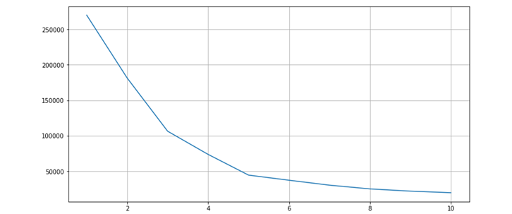
The Elbow method is used to find out the optimal value to be used in Kmeans In the line chart it resembles the arm with the elbow. The inflection in the curve resembles the underlined model that fits best at that point. So now we will use the elbow method to find out the number of clusters needed. We will first we will import means from sklearn lib and use wcss formula WCSS measures the sum of distances of observations from their cluster centroids which is given by the below formula.

where Yi is centroid for observation Xi. The main goal is to maximize the number of clusters and in limiting cases each data point becomes its own cluster centroid.

so the code to find the line chart is:

from sklearn.cluster import KMeans
wcss=[] #Within cluster sum of squares

for i in range(1,11):
kmeans=KMeans(n_clusters=i , init='k-means++',random_state=0)
kmeans.fit(x)
wcss.append(kmeans.inertia_)

plt.figure(figsize=(12,6))
plt.grid()
plt.plot(range(1,11),wcss)
plt.xlabel('KValue')
plt.xticks(np.arange(1,11,1))
plt.ylabel('WCSS')
plt.show()

From the obtained graph we can observe that at point 5 there is a maximum inflection in the curve. So we can use 5 clusters in K means algorithm

KMeans Algorithm

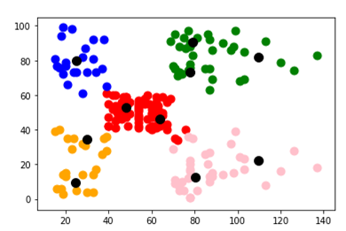
As we already know the number of clusters that are required is 5.Now Finally I made a plot to visualize the spending score of the customers with their annual income. The data points are separated into 5 classes which are represented in different colors as shown in the plot.

The code is as follows:

kmeansmodel=KMeans(n_clusters=5, init='k-means++', random_state=0)
y_kmeans=kmeansmodel.fit_predict(x)
plt.scatter(x[y_kmeans==0,0],x[y_kmeans==0,1],s=80,c='red',label='customer1')
plt.scatter(x[y_kmeans==1,0],x[y_kmeans==1,1],s=80,c='blue',label='customer2')
plt.scatter(x[y_kmeans==2,0],x[y_kmeans==2,1],s=80,c='green',label='customer3')
plt.scatter(x[y_kmeans==3,0],x[y_kmeans==3,1],s=80,c='orange',label='customer4')
plt.scatter(x[y_kmeans==4,0],x[y_kmeans==4,1],s=80,c='pink',label='customer5')
plt.scatter(kmeans.cluster_centers_[:,0],kmeans.cluster_centers_[:,1],s=100,c="black",label="centroids")
plt.title(str('cluster of customers'))
plt.xlabel(str('Annual Income'))
plt.ylabel(str('Spending Scores'))
plt.legend()
plt.show()

Here each customer represents one color customer1 as red, customer 2 as blue, customer3 as green, customer4 as orange, and customer5 as pink. The black dots represent the centroids of the cluster.

We have classified the customers into 5 clusters through which we can see that customer1 is having average spending scores with the average income so this range of customers can be targeted in order to increase sales

Summary

K means clustering is one of the most popular clustering algorithms and usually the first thing practitioners apply when solving clustering tasks to get an idea of the structure of the dataset. The goal of K means is to group data points into distinct non-overlapping subgroups. One of the major applications of K means clustering is the segmentation of customers to get a better understanding of them which in turn could be used to increase the revenue of the company

Customer Segmentation using Python in Machine Learning