Support Vector Machine(SVM) In Machine Learning

Introduction to Support vector machine

In the Machine Learning series, following a bunch of articles, in this article, we are going to learn about Support Vector Machine Algorithm in detail. In most of the tasks machine learning models handle like classifying images, handling large amounts of data, and predicting future values based on current values, we can choose different algorithms to fit the problem we are trying to solve. But do you know there’s an algorithm in machine learning that’ll handle just any data you can throw at it? Interesting right? Before starting with the algorithm get a quick overview of other machine learning algorithms.

What is a Support Vector Machine(SVM)?

Support Vector Machines are a set of supervised learning methods used for classification, regression, and outliers detection problems. All of these are very common tasks in machine learning and the Support vector machine is the best choice in many cases. Some of the examples where we can use them are, to detect cancerous cells, predict driving routes, face detection, handwriting recognition, image classification, Bioinformatics, etc.

The main point to keep in mind here is that these are just math equations tuned to give you the most accurate answer as quickly as possible. Support vector machines are different from other classification algorithms in the way they choose the decision boundary that maximizes the distance from the nearest data points of all the categories. The decision boundary created by SVM is called the maximum margin classifier or the maximum margin hyperplane.

Important terms in Support Vector Machine

Some of the important concepts in SVM which will be used frequently are as follows.

Hyperplane − It is a decision plane or space which is divided between a set of objects having different classes.
Support Vectors − Datapoints that are closest to the hyperplane are called support vectors. The separating line will be defined with the help of these data points.
Kernel – A kernel is a function used in SVM for helping to solve problems. They provide shortcuts to avoid complex calculations.
Margin − It may be defined as the gap between two lines on the closet data points of different classes. A large margin is considered a good margin and a small margin is considered as a bad margin.

How does SVM works?

A simple linear SVM classifier works by making a straight line between two groups of data. That means all of the data points on one side of the line will represent a particular category and the data points on the other side of the line will be put into a different category. This means there can be an infinite number of lines for us to choose from.

What makes the linear SVM algorithm better than some of the other algorithms, like k-nearest neighbors, is that it chooses the best line to classify the data points. The algorithm chooses the line that separates the data and is the furthest away from the closest data points as possible. If we select a hyperplane having a low margin then there is a high chance of misclassification.

An important function in the implementation of the SVM algorithm is the SVM kernel. It is a function that takes low dimensional input space and transforms it into a higher dimensional space. That is it converts a not separable problem or difficult classification problem into a separable problem. It is mostly useful in non-linear problems which we will discuss in the latter section.

Example of Support Vector Machine

SVM algorithm can be understood better with the following example. Suppose we want to build a model that can accurately identify whether the given fruit is an apple or banana. Then without any extra thought, we can decide that such a model can be built by the SVM algorithm.

We will first train our model with lots of images of apples and bananas so that it can learn about the different features of apples and bananas, and then we test it with new fruit. So as the support vector creates a decision boundary between these two data i.e., apple and banana, and chooses support vectors. On the basis of the support vectors, it will classify its category as an apple or banana. We can understand the example with the below diagram.

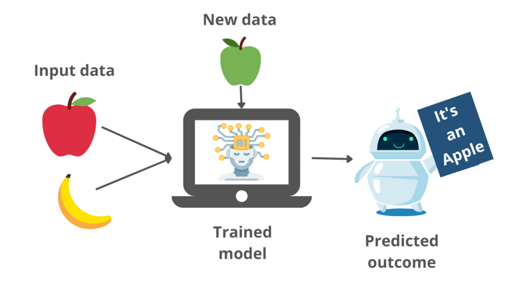
From the example image, we can get an overview of the working of the SVM model. The model classifies the new input as an apple with the help of features it understood with the training samples.

Types of Support vector Machine

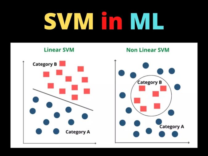
Support vector Machines can be of two types based on the type of the data. They are Linear SVM and Nonlinear SVM.

Linear SVM

Linear SVM is used in the case of linearly separable data. It means if a dataset can be classified into two classes by using a straight line, then such data is termed linearly separable data, and we can use the Linear SVM classifier. The formula of the linear kernel is as below which says that the product between two vectors is the sum of the multiplication of each pair of input values.

Linear Kernel formula in Support vector machine

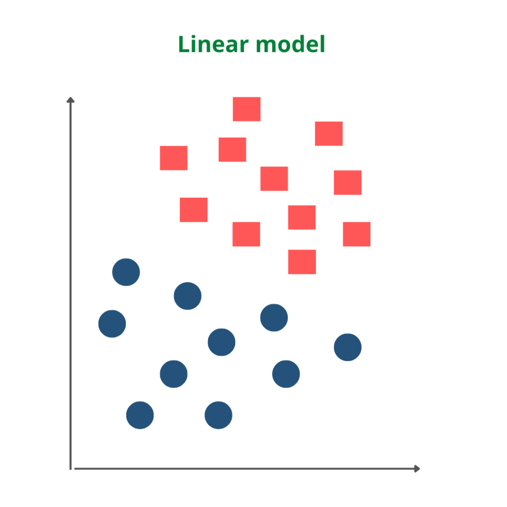
The working of the Linear SVM algorithm can be understood by using an example. Suppose we have a dataset that has two categories of data represented by blue and red. We want a classifier that can classify the pair of coordinates in either red or blue, which is plotted as follows.

Non-linear SVM

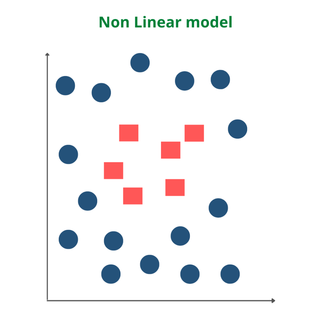
Non-Linear SVM is used in the case of non-linearly separated data. It means if a straight line cannot classify a dataset, then such data is termed non-linear data, and we can use the Non-linear SVM classifier.

Support vector machine Support Vector Machine(SVM) in Machine Learning In the Machine Learning series, following a bunch of articles, in this article, we are going to learn about Support Vector Machine Algorithm in detail. In most of the tasks machine learning models handle like classifying images, handling large amounts of data, and predicting future values based on current values, we can choose different algorithms to fit the problem we are trying to solve. But do you know there's an algorithm in machine learning that'll handle just any data you can throw at it? Interesting right? Before starting with the algorithm get a quick overview of other machine learning algorithms.

The working of the Non-Linear SVM algorithm can be understood by using an example. Suppose we have a dataset that has two categories of data represented by blue and red. We want a classifier that can classify the pair of coordinates in either red or blue, which is plotted as follows.

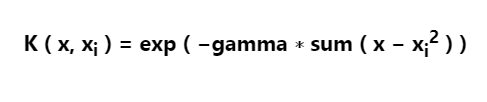
Radial Basis Kernel(RBF) is a kernel function that is used to find a non-linear classifier or regression line. RBF kernel, mostly used in SVM classification, maps input space in indefinite dimensional space.

So we got to know the process of segregating the two classes with a hyper-plane. Now, the question is how can we identify the right hyper-plane? Well, the answer to this is select the hyperplane which segregates the two categories in a better way.

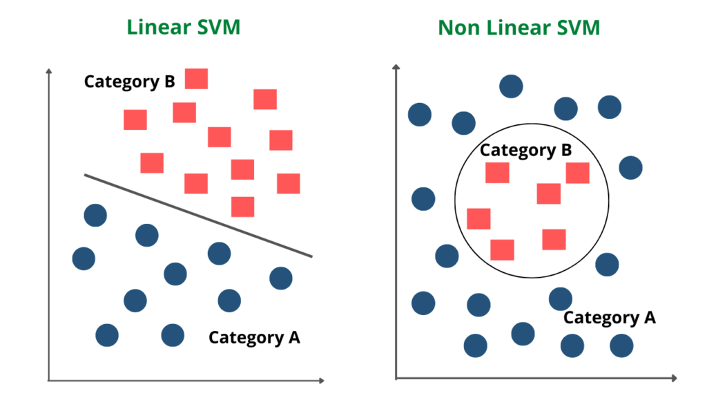
Linear and Non-linear Support vector machine

From the above image, we can understand the major difference between the linear and non-linear SVM types.

Implementation of Support Vector Machine in Python

We’ll start the implementation of the Support Vector Machine, by importing a few libraries that will be useful for our project.

#Importing the required libraries
import pandas as pd
import numpy as np
from sklearn import svm, datasets
from sklearn.svm import SVC
import matplotlib.pyplot as plt

Next, we will load our dataset into the code. For the implementation of our SVM model, we can use the iris dataset present in the sklearn library. After loading the data, while assigning the dependent and outcome variable, we only take the first two features to make our model simple.

#Loading the iris dataset
data = datasets.load_iris()

#Independent and dependent variables
X = data.data[:, :2]
Y = data.target

# Create a mesh to plot 
x_min, x_max = X[:, 0].min() - 1, X[:, 0].max() + 1
y_min, y_max = X[:, 1].min() - 1, X[:, 1].max() + 1
h = (x_max / x_min)/100
xx, yy = np.meshgrid(np.arange(x_min, x_max, h), np.arange(y_min, y_max, h))
X_plot = np.c_[xx.ravel(), yy.ravel()]

Let’s provide the value of the regularization parameter and create the SVM classifier object for the linear kernel.

#SVM regularization parameter
C=1.0

#Creating SVM classifier object for the linear kernel
svc_classifier = svm.SVC(kernel='linear', C=C).fit(X, y)

Z = svc_classifier.predict(X_plot)
Z = Z.reshape(xx.shape)

#Plotting the data
plt.figure(figsize=(15, 5))
plt.subplot(121)
plt.contourf(xx, yy, Z, cmap=plt.cm.tab10, alpha=0.3)
plt.scatter(X[:, 0], X[:, 1], c=y, cmap=plt.cm.Set1)
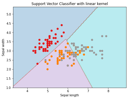
plt.xlabel('Sepal length')
plt.ylabel('Sepal width')
plt.xlim(xx.min(), xx.max())
plt.title('Support Vector Classifier with linear kernel')

Output

#SVM Regularization parameter 
C=1.0

#Creating SVM classifier object for the rbf kernel
svc_classifier = svm.SVC(kernel = 'rbf', gamma ='auto',C = C).fit(X, Y)

Z = svc_classifier.predict(X_plot)
Z = Z.reshape(xx.shape)

#Plotting the data
plt.figure(figsize=(15, 5))
plt.subplot(121)
plt.contourf(xx, yy, Z, cmap = plt.cm.tab10, alpha = 0.3)
plt.scatter(X[:, 0], X[:, 1], c = y, cmap = plt.cm.Set1)
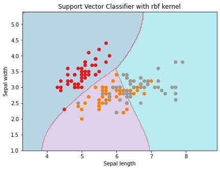
plt.xlabel('Sepal length')
plt.ylabel('Sepal width')
plt.xlim(xx.min(), xx.max())
plt.title('Support Vector Classifier with rbf kernel')

Output

Advantages of SVM

A support vector machine uses a subset of training points in the decision function called support vectors which makes it memory efficient.
It is effective in cases where the number of features is greater than the number of data points.
Support vector machine is effective on datasets with multiple features.
In this algorithm, different kernel functions can be specified for the decision function. We can also use custom kernels.

Disadvantages of SVM

The support vector machine algorithm works best on small data sets because of its high training time.
If the number of features is a lot bigger than the number of data points, avoiding over-fitting when choosing kernel functions and regularization term is crucial.
SVM doesn’t provide probability estimates, they are calculated using cross-validation.

Conclusion

In this article, we gained an overview of a Machine learning algorithm, Support Vector Machine in detail. We discussed its working, the important parameters, implementation in python, and finally its pros and cons. You can use the SVM algorithm for your model and analyze the power of this model by tuning the parameters.

Thank you for visiting our website.

Best 100+ Python Projects with source code

Also Read:

Support Vector Machine(SVM) in Machine Learning