In the last tutorial, we learned about our first ML algorithm called Linear Regression. We did it using an approach called Ordinary Least Squares, but there is another way to approach it. It is an approach that becomes the basis of Neural Networks, and it’s called Gradient Descent. And don’t get intimidated by the name because the approach is actually quite easy and we’ll understand how to implement it using sklearn too.
It’s recommended that you know the basics of multivariable calculus, if you are not familiar with it you can learn it here. It’ll be better if you understand Linear Regression Intuition, you can read our tutorial about it here.
The Intuition Behind Gradient Descent
So in machine learning, we usually try to optimize our algorithms like we try to adjust the parameters of the algorithm in order to achieve the optimal parameters that give us the minimum value of the loss function. So where does Gradient Descent helps in optimization, and more importantly, what does it do?
Gradient Descent is an optimization algorithm that is used to find the local minima of a differentiable function.
If the above statement didn’t make much sense it’s fine I’ll break it down. The first part says Gradient Descent is an optimization algorithm which means we can use it to optimize our model parameters we’ll understand how but now it’s clear why we need it.
The second part says that it is used to find the local minima of a differentiable function. Well…..that’s a big statement. Let’s start by understanding what exactly a differentiable function is. Well simply put a differentiable function is a function that can be differentiated and graphically its function whose graph is smooth and doesn’t have a break, angle, or cusp. Refer to the picture below to understand it a bit clearer.

Now as you can see the graph with that pointy angle thing in (0,0) is not differentiable and the smooth curve on the left is. Now refer to the following image for a refresher on local and global minima and maxima.

Now that we have everything cleared out let’s start by understanding gradient descent with a classic example of the mountaineer. So let’s imagine that we have our friend john who reached the top of Mount Everest. Wow, that’s something to be proud of but now he needs to reach the bottom so John starts taking steps in the direction that point to the bottom of the mountain something like this:-
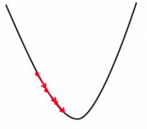
Now at each step, he had multiple directions to choose to take a step in but he chose to take the steps in the direction that leads to the bottom. If you’re familiar with multivariable calculus you’ll know that gradient is the value that gives you the direction of the steepest increase and its negative value gives you the direction of the step that decreases the value of the function quickly or the steepest descent.
Gradient Descent starts with random inputs and starts to modify them in such a way that they get closer to the nearest local minima after each step. But won’t it be better to achieve global minima? It’ll be but gradient descent can’t, gradient descent can only the nearest local minima. And as you might have guessed if a function has multiple local minima then the one chosen by Gradient Descent depends on the random input we choose at the beginning.
Hence in a nutshell the idea behind Gradient Descent is to take the steps in the direction of the steepest decrease,i.e. the opposite direction of the gradient, of the function at the current point.
But what is our function? What is its input? If we can’t achieve global minima then how does gradient descent optimize it?
Linear Regression using Gradient Descent
If you’ve read the previous article you’ll know that in Linear Regression we need to find the line that best fits the curve. That line was given by the following Hypothesis:-

our aim was to find the parameters θ0, θ1,…,θn. Now in OLS we simply had a formula that when fed the input found the θ matrix. But in gradient descent, we start by taking the random values of the parameters and then keep on modifying them until we find the value of parameters close to the local minimum of the function. WAIT! What is this function?
Well, my bad let me explain. The aim of linear regression is to find the best fit line but how do you define the best fit line? Well, the best-fit line was the line that when placed in the scatter plot had all the points as close to it as possible. But how do you measure this mathematically?
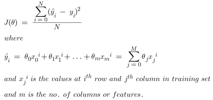
We can define a function to find out how well our line’s predictions are w.r.t. to the training set and for that we’ll use a metric called Mean Squared Error or MSE for short. Wow, that’s a weird name. Let me explain. Mean squared error is defined as the mean of the sum of the square difference between the predicted value of the target and the actual value of the target. It is calculated with the following formula:-

And this is the function whose value we have to minimize using Gradient Descent. In short, we have to find the value of the parameters closest to the local minima of the MSE function.
But local minima differ based on the value of starting point of parameters? Yes and that’s why we try to use a loss function that has only one local minimum and that local minimum is the global minimum. So no matter the starting point we’ll just be stepping in the direction of the global minimum.
MSE fits the description it has only one minimum and that is the global minimum. Now that we have the above stuff cleared let’s start talking about the steps in Gradient Descent.
Step 1: Specifying Initial Parameters
We start by randomly assigning values to our parameters. This will be the starting point in the curve, you can assign all the values as 0 or randomly assign them any values it’s up to you.
Step 2: Find Partial Derivative of Cost Function
To execute the gradient descent step you need to find the partial derivation of the cost function w.r.t. to each parameter. Calculating a partial derivative is similar to normal derivation except in this case we only calculate only the variable w.r.t. whom the partial derivative is being calculated and treat all other variables as constant. See the following example to understand better:-

As you can see in the partial derivative w.r.t. x we only took the derivative of the first term and treated y and z as constant and did the same for the partial derivative w.r.t. y where we took the derivative of the second term and treated x and z constant.
Now let’s calculate the derivative of our loss function we’ll call J(θ) for simplicity. J(θ) is nothing but the MSE function.
As we can see the predicted value, ŷ depends on the parameters
Step 3: The Gradient Descent Step
Now that we have our partial derivative we are all set to do our gradient descent step. So a typical gradient descent step looks like this:-

Great, that means at each iteration of Gradient Descent we update our parameters by subtracting the product of our partial derivative and that weird alpha symbol from it. But you might be confused regarding what that alpha is used for. That alpha is a vital hyperparameter called the Learning Rate. It basically defines how fast we achieve convergence or local minima point.
If the learning rate is too low then the convergence will be slow and if it’s too high the value of loss might overshoot. Hence it’s important to find an optimal learning rate. Usually, we start from 0.1 and keep updating it by dividing it by 10 until the optimal rate is found. Like : 0.1, 0.01, 0.001, …
Step 4: Repeat until Convergence
Repeat step 3 for x epochs or iterations. Assuming the learning rate is optimal with each epoch your training loss keeps reducing.
Gradient Descent using sklearn
In sklearn, Linear Regression in linear_model uses OLS to find the values of parameters but to use Linear Regression using Gradient Descent we use SGDRegressor present in linear_model. SGD stands for Stochastic Gradient Descent. We’ll use the diabetes dataset present in sklearn, in that dataset is a dictionary with features matrix under key data and target vector under key target. So let’s start by loading the data.
#Importing the libraries
import numpy as np
from sklearn.datasets import load_diabetes

#Loading the diabetes dataset
diabetes = load_diabetes()

X = diabetes.data
Y = diabetes.target
Now that we have our data let’s create our SGDRegressor object and train it on the data. To train the data we use the fit() method as usual. max_iter is used to define the max epochs and alpha is used to set the learning rate.
#Loading the data to the model
from sklearn.linear_model import SGDRegressor
reg = SGDRegressor(max_iter= 10000, alpha=0.0001)
reg.fit(X,Y)
Now let’s check how accurate the model is by finding the RMSE value. For this model, it came out to be 54.03.
#Calculating the mean square error
from sklearn.metrics import mean_squared_error
y_pred = reg.predict(X)
print(np.sqrt(mean_squared_error(Y, y_pred)))
Gradient Descent Variants
There are two categories of Gradient descent which include Stochastic Gradient Descent and Batch Gradient Descent
Stochiastic Gradient Descent
In this method, the parameters are updated with the computed gradient for each training point at a time. So, at a time a single training point is used and its corresponding loss is computed. The parameters are updated after every training sample.
Algorithm for stochastic gradient descent
As mentioned, this algorithm takes one example per iteration. Let (x(I), y(I) be the training sample

Stochastic Gradient Descent Advantages
- It is computationally fast as only one sample is processed at a time.
- For larger datasets, it can converge faster as it causes updates to the parameters more frequently
- Due to frequent updates, the steps taken towards the minima of the loss function have oscillations which can help to get out of local minimums of the loss function
Stochastic Gradient Descent Disadvantages
- Due to frequent updates, the steps taken towards the minima are very noisy. This can often lead the gradient descent into other directions.
- It loses the advantage of vectorized operations as it deals with only a single example at a time
- Frequent updates are computationally expensive due to using all resources for processing one training sample at a time
Batch Gradient Descent
The concept of carrying out batch gradient descent is the same as stochastic gradient descent. The difference is that instead of updating the parameters after using every training point, the parameters are instead updated only once i.e. after loss for all the training points is calculated.
Algorithm for batch gradient descent
Let hθ(x) be the hypothesis for linear regression. Then, the cost function is given by:

Let Σ represents the sum of all training examples from i=1 to m. Where xj(i) represents the jth feature of the ith training example. If m is large it will take a long time. So, Batch gradient descent is not recommended for long datasets.
Batch Gradient Descent Advantages
- It can benefit from vectorization which increases the speed of processing all training samples together
- It produces a more stable gradient descent convergence and stable error gradient than stochastic gradient descent
- It is computationally efficient as all computer resources are not being used to process a single sample
Batch Gradient Descent Disadvantages
- Depending on computer resources it can take too long for processing all the training samples as a batch
- The entire training set can be too large to process in the memory due to which additional memory might be needed
Thanks for reading
I hope you enjoyed learning and got what you need.
Comment if you have any queries or if you found something wrong in this article.
Also Read:
- Flower classification using CNNYou know how machine learning is developing and emerging daily to provide efficient and hurdle-free solutions to day-to-day problems. It covers all possible solutions, from building recommendation systems to predicting something. In this article, we are discussing one such machine-learning classification application i.e. Flower classification using CNN. We all come across a number of flowers…
- Music Recommendation System in Machine LearningIn this article, we are discussing a music recommendation system using machine learning techniques briefly. Introduction You love listening to music right? Imagine hearing your favorite song on any online music platform let’s say Spotify. Suppose that the song’s finished, what now? Yes, the next song gets played automatically. Have you ever imagined, how so?…
- Top 15 Python Libraries For Data Science in 2022Introduction In this informative article, we look at the most important Python Libraries For Data Science and explain how their distinct features may help you develop your data science knowledge. Python has a rich data science library environment. It’s almost impossible to cover everything in a single article. As a consequence, we’ve compiled a list…
- Top 15 Python Libraries For Machine Learning in 2022Introduction In today’s digital environment, artificial intelligence (AI) and machine learning (ML) are getting more and more popular. Because of their growing popularity, machine learning technologies and algorithms should be mastered by IT workers. Specifically, Python machine learning libraries are what we are investigating today. We give individuals a head start on the new year…
- Setup and Run Machine Learning in Visual Studio CodeIn this article, we are going to discuss how we can really run our machine learning in Visual Studio Code. Generally, most machine learning projects are developed as ‘.ipynb’ in Jupyter notebook or Google Collaboratory. However, Visual Studio Code is powerful among programming code editors, and also possesses the facility to run ML or Data…
- Diabetes prediction using Machine LearningIn this article, we are going to build a project on Diabetes Prediction using Machine Learning. Machine Learning is very useful in the medical field to detect many diseases in their early stage. Diabetes prediction is one such Machine Learning model which helps to detect diabetes in humans. Also, we will see how to Deploy…
- 15 Deep Learning Projects for Final yearIntroduction In this tutorial, we are going to learn about Deep Learning Projects for Final year students. It contains all the beginner, intermediate and advanced level project ideas as well as an understanding of what is deep learning and the applications of deep learning. What is Deep Learning? Deep learning is basically the subset of…
- Machine Learning Scenario-Based QuestionsHere, we will be talking about some popular Data Science and Machine Learning Scenario-Based Questions that must be covered while preparing for the interview. We have tried to select the best scenario-based machine learning interview questions which should help our readers in the best ways. Let’s start, Question 1: Assume that you have to achieve…
- Customer Behaviour Analysis – Machine Learning and PythonIntroduction A company runs successfully due to its customers. Understanding the need of customers and fulfilling them through the products is the aim of the company. Most successful businesses achieved the heights by knowing the need of customers and dynamically changing their strategies and development process. Customer Behaviour Analysis is as important as a customer…
- NxNxN Matrix in Python 3A 3d matrix(NxNxN) can be created in Python using lists or NumPy. Numpy provides us with an easier and more efficient way of creating and handling 3d matrices. We will look at the different operations we can provide on a 3d matrix i.e. NxNxN Matrix in Python 3 using NumPy. Create an NxNxN Matrix in…
- 3 V’s of Big dataIn this article, we will explore the 3 V’s of Big data. Big data is one of the most trending topics in the last two decades. It is due to the massive amount of data that has been produced as well as consumed by everyone across the globe. Major evolution in the internet during the…
- Naive Bayes in Machine LearningIn the Machine Learning series, following a bunch of articles, in this article, we are going to learn about the Naive Bayes Algorithm in detail. This algorithm is simple as well as efficient in most cases. Before starting with the algorithm get a quick overview of other machine learning algorithms. What is Naive Bayes? Naive Bayes…
- Automate Data Mining With PythonIntroduction Data mining is one of the most crucial steps in Data Science. To drive meaningful insights from data to take business decisions, it is very important to mine the data. Deleting or ignoring unnecessary and unavailable parts of data and focusing on the correct and right data is beneficial, and more if required in…
- Support Vector Machine(SVM) in Machine LearningIntroduction to Support vector machine In the Machine Learning series, following a bunch of articles, in this article, we are going to learn about Support Vector Machine Algorithm in detail. In most of the tasks machine learning models handle like classifying images, handling large amounts of data, and predicting future values based on current values,…
- Convert ipynb to PythonThis article is all about learning how to Convert ipynb to Python. There is no doubt that Python is the most widely used and acceptable language and the number of different ways one can code in Python is uncountable. One of the most preferred ways is by coding in Jupyter Notebooks. This allows a user…
- Data Science Projects for Final YearDo you plan to complete your data science course this year? If so, one of the criteria for receiving your degree can be a data analytics project. Picking the best Data Science Projects for Final Year might be difficult. Many of them have a high learning curve, which might not be the best option if…
- Multiclass Classification in Machine LearningIntroduction The fact that you’re reading this article is evidence of the fact that you’ve finally realised that classification problems in real life are rarely limited to a binary choice of ‘yes’ and ‘no’, or ‘this’ and ‘that’. If the number of classes that the tuples can be classified into exceeds two, the classification is…
