Introduction
Data mining is one of the most crucial steps in Data Science. To drive meaningful insights from data to take business decisions, it is very important to mine the data. Deleting or ignoring unnecessary and unavailable parts of data and focusing on the correct and right data is beneficial, and more if required in the world of Data Science.
In this blog, we’ll understand how to Automate Data Mining With Python.
What is Data Mining?
Well, data mining can be defined in so many ways but the central idea of all is, the processing and analyzing the raw data into information, into meaningful data.
It is the process of extracting potentially useful information from the data. The process of structuring, analyzing, and formulating massive amounts of raw data in order to find patterns and anomalies through mathematical and computational algorithms is called Data Mining.
Python supports a wide set of scientific computational libraries, hence, it is one of the most popular and most powerful tools as well to mining data. Data Mining includes:
- Visualizing the data
- Classifying the data
- Discovering the relationship between the data
- Reducing the data
- Analyzing the data
We’ll be looking practically into these steps.
The 5 top data mining techniques used by companies and individuals are
- MapReduce
- Clustering
- Link Analysis
- Recommendation Systems
- Frequent Itemset Analysis.
Automate Data Mining With Python
The Dataset
Let’s dive into the practical steps of data mining in Python. For this, we’ll mine the iris dataset. You can find the dataset here. This is the archive, make sure to unarchive and extract the iris.csv file.
Data Importing and Data Visualization
Import the file into google colab or jupyter.
urllib2 is a python2 library, from python 3 and its next versions, it is urllib.request
import urllib.request as urllib2
localFile = open('Iris.csv','r')
localFile.close()
The CSV file contains the iris dataset, which is a multivariate dataset that consists of 50 samples from each of three species of Iris flowers (Iris setosa, Iris virginica, and Iris versicolor). Each sample has four features (or variables) that are the length and the width of the sepal and petal, in centimeters.
CSV files are easy to parse. Parsing using the CSV can be easily parsed using the function genfromtxt of the NumPy library:
from numpy import genfromtxt, zeros
# read the first 4 columns
data = genfromtxt('Iris.csv',delimiter=',',usecols=(0,1,2,3))
# read the fifth column
target = genfromtxt('Iris.csv',delimiter=',',usecols=(4),dtype=str)
Now to parse, we have created a matrix with the features and a vector that contains the classes.
We can look for the classes as:
set(target)

#Output:
{'Iris-setosa', 'Iris-versicolor', 'Iris-virginica'}
We can confirm the size of our dataset by looking at the shape of the data structures we loaded:
print(data.shape)
#Output

(150,4)

print(target.shape)
#Output
(150,)
Now for the visualization, we’ll use matplotlib.
import matplotlib.pyplot as plt
plt.plot(data[target=='Iris-setosa',0],data[target=='Iris-setosa',2],'bo')
plt.plot(data[target=='Iris-versicolor',0],data[target=='Iris-versicolor',2],'ro')
plt.plot(data[target=='Iris-virginica',0],data[target=='Iris-virginica',2],'go')
plt.show()
The pyplot plots the graph for sepal length against sepal width as,
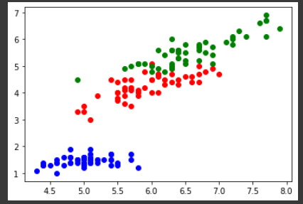
In the above graph, the blue points represent the samples that belong to the specie setosa, the red ones represent Versicolor and the green ones represent virginica.
We can represent the same in the histogram.
import matplotlib.pyplot as plt
xmin = min(data[1:,0])
xmax = max(data[1:,0])
plt.figure()
plt.subplot(411) # distribution of the setosa class (1st, on the top)
plt.hist(data[target=='Iris-setosa',0],color='b',alpha=.7)
plt.xlim(xmin,xmax)
plt.subplot(412) # distribution of the versicolor class (2nd)
plt.hist(data[target=='Iris-versicolor',0],color='r',alpha=.7)
plt.xlim(xmin,xmax)
plt.subplot(413) # distribution of the virginica class (3rd)
plt.hist(data[target=='Iris-virginica',0],color='g',alpha=.7)
plt.xlim(xmin,xmax)
plt.subplot(414) # global histogram (4th, on the bottom)
plt.hist(data[:,0],color='y',alpha=.7)
plt.xlim(xmin,xmax)
plt.show()
From the above histogram, we can observe that, on average, the Iris setosa flowers have a smaller sepal length compared to the Iris virginica.
Classification
Classification is the process of taking a classifier built with such a training dataset and running it on unknown data to determine class membership for the unknown samples.
We will use Gaussian Naive Bayes to identify iris flowers as setosa, Versicolor, or virginca from the loaded dataset.
We convert the vector of strings that contain the class into integers:
t = zeros(len(target))
t[target == 'Iris-setosa'] = 1
t[target == 'Iris-versicolor'] = 2
t[target == 'Iris-virginica'] = 3
Now we are ready to instantiate and train our classifier:
from sklearn.naive_bayes import GaussianNB
classifier = GaussianNB()
classifier.fit(data,t)
The classification can be done with the predict method:
print(classifier.predict(data[0]))
#Output
[ 1.]

print(t[0])
#Output
1
Train and Test Data
from sklearn import cross_validation
train, test, t_train, t_test = cross_validation.train_test_split(data, t, …
test_size=0.4, random_state=0)
Now the dataset has been categorized into train and test data. Test data occupies 40% of the data available in the dataset.
With this data we can again train the classifier and print its accuracy:
classifier.fit(train,t_train) # train
print(classifier.score(test,t_test))# test

#Output
0.93333333333333335
We have achieved 93% of accuracy. Accuracy is nothing but the measure of proportions of the total number of predictions that are correct.
Also, with the help of the confusion matrix, we can analyze the performance of the classifier.
Clustering
Clustering is used when the data is not labeled. In other words, where we have to form the groups of data on the basis of likeness or similarity. Clustering falls under unsupervised learning and one of the major used algorithms for it is the k-means clustering algorithm.
We can run this algo on our data as:
from sklearn.cluster import KMeans
kmeans = KMeans(k=3, init='random') # initialization
kmeans.fit(data)
The parameter ‘k’ defines the number of clusters that are to be formed. We can use this model on our data as,
c = kmeans.predict(data)We can evaluate the results of clustering, comparing it with previous using completeness and homogeneity scores.
from sklearn.metrics import completeness_score, homogeneity_score
print(completeness_score(t,c))

#Output
0.7649861514489815

print(homogeneity_score(t,c))

#Output
0.7514854021988338
When the majority of the data points of a given class are elements of the same cluster, the completeness score becomes 1 and when all the clusters contain data points of a single class, the homogeneity score turns 1.
Regression
Regression is a method for defining functional relationships among variables that can be used to make predictions. Linear regression analysis is used to predict the value of a variable based on the value of another variable. The variable you want to predict is called the dependent variable. The variable you are using to predict the other variable’s value is called the independent variable.
To understand, we can build a synthetic dataset and perform regression over it:
from numpy.random import rand
x = rand(50,1) #independent variable
y = x*x*x+rand(50,1)/5 #dependant variable
Here now we can use the LinearRegression model from sklear.linear_model. This model calculates the best-fitting line for the observed data by minimizing the sum of the squares of the vertical deviations from each data point to the line.
from sklearn.linear_model import LinearRegression
linreg = LinearRegression()
linreg.fit(x,y)
We can plot this line over the data points as,
from numpy import linspace, matrix
import matplotlib.pyplot as plt
xx = linspace(0,1,40)
plt.plot(x,y,'o',xx,linreg.predict(matrix(xx).T),'--r')
plt.show()
From the visual graph, we can observe that the line goes through the center of our data and identifies the increasing trend.
Using mean squared error, we can calculate prediction accuracy. This metric measures the expected squared distance between the prediction and the true data. It is 0 when the prediction is accurate.
from sklearn.metrics import mean_squared_error
print(mean_squared_error(linreg.predict(x),y))

#Output
0.014552409677571747
Dimensionality Reduction
We can only plot 3 dimensions on the axis as the view of data. But sometimes dataset might be of a number of dimensions. Hence it is required to embed these dimensions to up to 3.
One of the most popular techniques for dimensionality reduction is the Principal Component Analysis (PCA). This technique transforms the variables of the data into equal or smaller numbers of uncorrelated variables. These variables are called Principal Components or PC’s.
Import PCA from sklearn.decomposition, we can instantiate a PCA object which we can use to compute the first two PCs.
So these were some of the data mining techniques in Python.
Data mining encompasses a number of predictive modeling techniques and we can use a variety of data mining software. Python’s ease of use coupled with many of its powerful modules makes it a versatile tool for data mining and analysis.
Data mining is different from KDD (Knowledge Discovery in Data).
The top data mining algorithms are:
- SVM (Support Vector Machine)
- Apriori Algorithm
- PCA
- Collaborative filtering
- K-means
Conclusion
Automate Data Mining With Python can be very useful and time-saving in many cases. Classification, Clustering, Regression, and Association Rules are some of the popular Python data mining tools. Data mining is an essential part of Data Science so you should practice data mining as much as possible.
We hope this article on “Automate Data Mining With Python” will help you.
Thank you for visiting our website.
Also Read:
- Flower classification using CNN
- Music Recommendation System in Machine Learning
- Top 15 Machine Learning Projects in Python with source code
- Gender Recognition by Voice using Python
- Top 15 Python Libraries For Data Science in 2022
- Top 15 Python Libraries For Machine Learning in 2022
- Setup and Run Machine Learning in Visual Studio Code
- Diabetes prediction using Machine Learning
- 15 Deep Learning Projects for Final year
- Machine Learning Scenario-Based Questions
- Customer Behaviour Analysis – Machine Learning and Python
- NxNxN Matrix in Python 3
- 3 V’s of Big data
- Naive Bayes in Machine Learning
- Automate Data Mining With Python
- Support Vector Machine(SVM) in Machine Learning
- Convert ipynb to Python
- Data Science Projects for Final Year
- Multiclass Classification in Machine Learning
- Movie Recommendation System: with Streamlit and Python-ML
- Getting Started with Seaborn: Install, Import, and Usage
- List of Machine Learning Algorithms
- Recommendation engine in Machine Learning
- Machine Learning Projects for Final Year
- ML Systems
- Python Derivative Calculator
- Mathematics for Machine Learning
- Data Science Homework Help – Get The Assistance You Need
- How to Ace Your Machine Learning Assignment – A Guide for Beginners
- Top 10 Resources to Find Machine Learning Datasets in 2022