We will discuss Logistic Regression: Regression Model for Classification in this article, but let us see what we did in the past couple of articles, we discussed how we can use an ML algorithm called Linear Regression to predict continuous values by training it over a training dataset.
We talked about 2 ways to do this, Ordinary Least Squares and Gradient Descent. But for classification problems, we can’t use it and we’ll see why in a short while. Hence we need another approach for classification problems as is so after tweaking Linear Regression a bit we can actually use it for classification problems and this approach is called Logistic Regression.
But before learning about logistic regression let’s understand why we need another algorithm for classification problems.
Linear Regression for Classification
So let’s talk about why can’t we just use linear regression for classification and why need another algorithm. So let’s take an example to understand it clearly.
Let’s say you are a doctor at X hospital and your job is to tell whether the tumor in the patient is malignant or benign. And now that you have this newfound power of machine learning you wish to exploit it here. So you pulled out the record of 5 people and that record consisted of the tumor size of the patient and tumor status i.e. 0 if benign and 1 if malignant. The data looked like the following:-
| Tumor Size | Tumor Status |
| 1 | 0 |
| 0.5 | 0 |
| 2 | 0 |
| 4 | 1 |
| 6 | 1 |
Now you used this data to train your linear regression model but you are intelligent and knew that the target value can be either 0 or 1 but your model will give you a continuous value, so you came up with the strategy to assume the values above 0.5 as 1 and below 0.5 as 0. With strategy all set you ran your regression model and got the following line as the best fit line:-
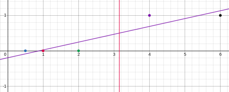
The purple line is the regression line and the red line is the line that intercepts the regression line at y = 0.5. Every point on the right of the red line suggests a malignant tumor and everything on the left of it represents a benign tumor. Let’s call this line the decision boundary. Great, problem solved? Well not yet, you took this model and took it to your ML expert friend to verify the results. Your friend rejected the approach itself which left you disappointed and angry. Your friend seeing your angry self got scared and explained the following. He gave you a new additional record entry to train one that looked like the following:-
| Tumor Size | Tumor Status |
| 1 | 0 |
| 0.5 | 0 |
| 2 | 0 |
| 4 | 1 |
| 6 | 1 |
| 15 | 1 |
Now your friend asked you to train the regression model on this data. You trained the model again and got the following results:-

Now you saw that the point (4,1) which was classified correctly by the previous model is now on the right side of the decision boundary i.e. it’s classified as benign even though it’s malignant. But this shouldn’t happen. Now our y>0.5 is malignant and doesn’t work anymore. To keep making correct predictions we need to change it to y>0.3 or something, but that is not how the algorithm should work. Logistic Regression seems to solve this problem by creating a new hypothesis i.e. passing this regression line equation into a sigmoid function. How? Let’s see!
Logistic Regression Intuition
Working of Logistic Regression is pre much the same as that of Linear Regression with an additional step. Linear Regression models predict the continuous value of the target which could be anything but in binary classification target variable only has 2 values i.e. usually 0 or 1.
It seems it would be better if our model could predict values between 0 and 1. But linear regression predicts values in interval (−∞,+∞), hence we need a way to map these predictions in the range [0,1]. This is precisely what the sigmoid function does. Sigmoid takes a value as an input and returns a value that lies between 0 and 1. The sigmoid function has the following equation and graph.

In order to map predicted values to probabilities, we use the sigmoid function. The function maps any real value into another value between 0 and 1. We use sigmoid to map predictions to probabilities. Now that we understand the sigmoid function let’s get an overview of how logistic regression works.
In logistic regression, we train our model the same way we try to find the best fit line that’ll help us make predictions the same way except for this time after we make the prediction from the regression line we’ll pass the prediction to the sigmoid function to map it between 0 and 1 and if it’s greater than 0.5 than it’ll be 1 else 0. And that’s usually how logistic regression works. Now that we know the procedure let’s understand the math a bit more.
Working of Logistic Regression
So in logistic regression, our hypothesis is a composite function of a sigmoid and linear function, let’s say S(x) is our sigmoid function and h(x) is our linear regression hypothesis, we’ll have our logistic regression hypothesis as the following:-
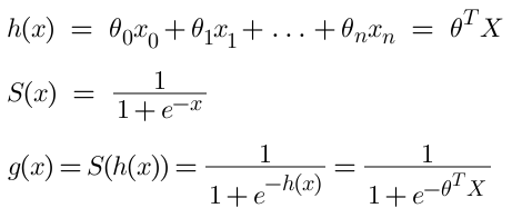
Now that we have a hypothesis to get the parameter for and to find the parameter it’s the same as linear regression we can use OLS to find the best fit line and be happy for the day. But for Gradient Descent we need a loss function to minimize, we can’t use MSE as we did in linear regression.
Intuitively, we want to assign more punishment when predicting 1 while the actual is 0 and when predicting 0 while the actual is 1. The loss function of logistic regression is doing this exactly which is called Logistic Loss.
Notice how I wrote loss(y, g(x)) instead of loss(y, ŷ), that because ŷ is the class value i.e. 0 or 1 and we have to improve the predicted probability for the corresponding feature i.e. g(x) our logistic regression hypothesis. If you didn’t understand then let me put it more simply, our hypothesis gives values between 0 and 1 the closer the value to 0 the more sure we are that the data belongs to class 0, and the closer the value to 1 the more sure we are that the data belongs to class 1. Hence we want our hypothesis to return a value much closer to 1 if the class is 1 and closer to 0 if the class is 0. That’s what we are aiming to improve.
Another advantage of this loss function is that although we are looking at it by y = 1 and y = 0 separately. Now that we have the hypothesis and loss function we can use gradient descent as usual to get the optimal parameters. Now let’s jump to the exciting stuff i.e. CODE!
Logistic Regression using sklearn
Logistic Regression is present in sklearn under linear_model. We’ll use the breast cancer dataset present in sklearn, that dataset is a dictionary with a features matrix under key data and target vector under key target. So let’s start by loading the data.
#Importing the required libraries
from sklearn.datasets import load_breast_cancer

#Loading the data
cancer = load_breast_cancer()

X = cancer.data
Y = cancer.target
So we have our data with us and while we are at it I want to introduce you to Model Validation more specifically to a function in sklearn called train_test_split. Our model will usually perform better on data it’s trained on because well it is the data it’s trained on. But it might happen that you are faced with the problem of overfitting or underfitting.
Overfitting means your model performs quite well on the training dataset but performs poorly on testing data. Underfitting means your model performed poorly on both training and testing data. If this happens you can tweak your hyperparameters or apply regularization to get better performance.
In order to determine if our model performs well on data other than training data, we can split our data into two parts, one that we’ll use to train our model called training data, and one that we’ll use to test the performance of our model called testing data. train_test_split does exactly that we give it our data and test_size i.e. ratio of data to be used as test data.
#Importing the train_test_split method
from sklearn.model_selection import train_test_split

#Splitting the data into training and testing data
x_train, x_test, y_train, y_test = train_test_split(X,Y, test_size = 0.3)
Now that we have our training and testing data let’s create our LogisticRegression object and train it on the training data. To train the data we use the fit() method like always. Let’s do it.
#Loading the data into the model
from sklearn.linear_model import LogisticRegression

clf = LogisticRegression()
clf.fit(x_train, y_train)
Now let’s check how accurate the model is by finding the accuracy score for the testing dataset. For this model, it came out to be 0.935 meaning that about 93.5% of predictions were correct.
#Importing the accuracy_score method
from sklearn.metrics import accuracy_score

#calculating the accuracy score
print(accuracy_score(y_test,clf.predict(x_test)))
Multiclass Classification
We’ve seen how logistic regression works but we can’t use the above approach for multiclass classification. But that doesn’t mean we can’t use it for multiclass classification, we can but just a bit differently. There are 2 techniques we can use to do multiclass classification using Logistic Regression: One vs All and One vs One.
One vs All
Let us say a data set has n classes, in One vs All we train n classifiers over ith class vs not the ith class. Let’s understand by example. Let us say we have to classify the animal into 3 categories Dog, Cat, and Rabbit based on the given data. We’ll train 3 separate classifiers in their respective classes:-
- Classifier 1: Dog vs not Dog
- Classifier 2: Cat vs not Cat
- Classifier 3: Rabbit vs not Rabbit
We’ll modify the training data by assigning the dog class the value 1 and the rest -1 and use it to train classifier 1 and do it similarly for classifiers 2 and 3. After training the models over their respective classes we’ll test them. Let’s suppose we passed the testing data for the dog class. What will happen is that this input will be passed in all classifiers and what we expect is that classifier 1 gives us a positive value and the rest give the negative value and since the dog classifier gave a positive value the predicted class is Dog.
One vs One
Let’s say a data set has n classes, in One vs All we train nC2 classifiers over the ith class vs the jth class. Let’s that the same example, we’ll again classify the animal into 3 categories Dog, Cat, and Rabbit based on given data. We’ll train 3 separate classifiers in their respective classes:-
- Classifier 1: Dog vs Cat
- Classifier 2: Cat vs Rabbit
- Classifier 3: Rabbit vs Dog
Each binary classifier predicts one class label. When we input the test data to the classifier, the model with the majority counts is concluded as a result. So if we try to predict dog class then Classifiers 1 and 3 will predict dog and since we got the dog as the predicted class in 2 out of 3 classifiers we’ll say that is our predicted class.
Assumptions of Logistic Regression
- Binary logistic regression requires the dependent variable to be binary and ordinal.
- It requires the observations to be independent of each other.
- It requires there to be little or no multicollinearity among the independenThanksables. This means that the independent variables should not be too highly correlated with each other.
- It typically requires a large sample size.
Comparison of Linear and Logistic Regression
Linear Regression and Logistic Regression are the two most common and well-known Machine Learning Algorithms that come under the supervised learning technique. Linear regression is used to predict the continuous dependent variable using a given set of independent variables. Logistic Regression is used to predict the categorical dependent variable using a given set of independent variables.
Since both algorithms are supervised, these algorithms use labeled datasets to make predictions. But the main difference between them is how they are being used. Linear Regression is used for solving Regression problems whereas Logistic Regression is used for solving Classification problems.

Linear regression provides a continuous output but Logistic regression provides discrete output. The purpose of Linear Regression is to find the best-fitted line while Logistic regression is one step ahead and fitting the line values to the sigmoid curve.
Advantages of Logistic Regression
- It is easier to implement, and interpret, and very efficient to train.
- Good accuracy for many simple data sets and it performs well when the dataset is linearly separable.
- It can interpret model coefficients as indicators of feature importance.
- Logistic regression is less inclined to over-fitting but it can overfit in high-dimensional datasets. One may consider Regularization (L1 and L2) techniques to avoid over-fitting in these scenarios.
Disadvantages of Logistic Regression
- It constructs linear boundaries.
- If the number of observations is lesser than the number of features, it should not be used, otherwise, it may lead to overfitting.
- It is tough to obtain complex relationships using it.
- Non-linear problems can’t be solved with it.
Credits: StatQuest with Josh Starmer
Thanks for reading
I hope you enjoyed learning and got what you need.
Comment if you have any queries or if you found something wrong in this article.
Also Read:
- Flower classification using CNNYou know how machine learning is developing and emerging daily to provide efficient and hurdle-free solutions to day-to-day problems. It covers all possible solutions, from building recommendation systems to predicting something. In this article, we are discussing one such machine-learning classification application i.e. Flower classification using CNN. We all come across a number of flowers…
- Music Recommendation System in Machine LearningIn this article, we are discussing a music recommendation system using machine learning techniques briefly. Introduction You love listening to music right? Imagine hearing your favorite song on any online music platform let’s say Spotify. Suppose that the song’s finished, what now? Yes, the next song gets played automatically. Have you ever imagined, how so?…
- Top 15 Python Libraries For Data Science in 2022Introduction In this informative article, we look at the most important Python Libraries For Data Science and explain how their distinct features may help you develop your data science knowledge. Python has a rich data science library environment. It’s almost impossible to cover everything in a single article. As a consequence, we’ve compiled a list…
- Top 15 Python Libraries For Machine Learning in 2022Introduction In today’s digital environment, artificial intelligence (AI) and machine learning (ML) are getting more and more popular. Because of their growing popularity, machine learning technologies and algorithms should be mastered by IT workers. Specifically, Python machine learning libraries are what we are investigating today. We give individuals a head start on the new year…
- Setup and Run Machine Learning in Visual Studio CodeIn this article, we are going to discuss how we can really run our machine learning in Visual Studio Code. Generally, most machine learning projects are developed as ‘.ipynb’ in Jupyter notebook or Google Collaboratory. However, Visual Studio Code is powerful among programming code editors, and also possesses the facility to run ML or Data…
- Diabetes prediction using Machine LearningIn this article, we are going to build a project on Diabetes Prediction using Machine Learning. Machine Learning is very useful in the medical field to detect many diseases in their early stage. Diabetes prediction is one such Machine Learning model which helps to detect diabetes in humans. Also, we will see how to Deploy…
- 15 Deep Learning Projects for Final yearIntroduction In this tutorial, we are going to learn about Deep Learning Projects for Final year students. It contains all the beginner, intermediate and advanced level project ideas as well as an understanding of what is deep learning and the applications of deep learning. What is Deep Learning? Deep learning is basically the subset of…
- Machine Learning Scenario-Based QuestionsHere, we will be talking about some popular Data Science and Machine Learning Scenario-Based Questions that must be covered while preparing for the interview. We have tried to select the best scenario-based machine learning interview questions which should help our readers in the best ways. Let’s start, Question 1: Assume that you have to achieve…
- Customer Behaviour Analysis – Machine Learning and PythonIntroduction A company runs successfully due to its customers. Understanding the need of customers and fulfilling them through the products is the aim of the company. Most successful businesses achieved the heights by knowing the need of customers and dynamically changing their strategies and development process. Customer Behaviour Analysis is as important as a customer…
- NxNxN Matrix in Python 3A 3d matrix(NxNxN) can be created in Python using lists or NumPy. Numpy provides us with an easier and more efficient way of creating and handling 3d matrices. We will look at the different operations we can provide on a 3d matrix i.e. NxNxN Matrix in Python 3 using NumPy. Create an NxNxN Matrix in…
- 3 V’s of Big dataIn this article, we will explore the 3 V’s of Big data. Big data is one of the most trending topics in the last two decades. It is due to the massive amount of data that has been produced as well as consumed by everyone across the globe. Major evolution in the internet during the…
- Naive Bayes in Machine LearningIn the Machine Learning series, following a bunch of articles, in this article, we are going to learn about the Naive Bayes Algorithm in detail. This algorithm is simple as well as efficient in most cases. Before starting with the algorithm get a quick overview of other machine learning algorithms. What is Naive Bayes? Naive Bayes…
- Automate Data Mining With PythonIntroduction Data mining is one of the most crucial steps in Data Science. To drive meaningful insights from data to take business decisions, it is very important to mine the data. Deleting or ignoring unnecessary and unavailable parts of data and focusing on the correct and right data is beneficial, and more if required in…
- Support Vector Machine(SVM) in Machine LearningIntroduction to Support vector machine In the Machine Learning series, following a bunch of articles, in this article, we are going to learn about Support Vector Machine Algorithm in detail. In most of the tasks machine learning models handle like classifying images, handling large amounts of data, and predicting future values based on current values,…
- Convert ipynb to PythonThis article is all about learning how to Convert ipynb to Python. There is no doubt that Python is the most widely used and acceptable language and the number of different ways one can code in Python is uncountable. One of the most preferred ways is by coding in Jupyter Notebooks. This allows a user…
- Data Science Projects for Final YearDo you plan to complete your data science course this year? If so, one of the criteria for receiving your degree can be a data analytics project. Picking the best Data Science Projects for Final Year might be difficult. Many of them have a high learning curve, which might not be the best option if…
- Multiclass Classification in Machine LearningIntroduction The fact that you’re reading this article is evidence of the fact that you’ve finally realised that classification problems in real life are rarely limited to a binary choice of ‘yes’ and ‘no’, or ‘this’ and ‘that’. If the number of classes that the tuples can be classified into exceeds two, the classification is…
