Hi guys! So until now, we’ve learned about how we can use libraries to play with data. We did data analysis on a real dataset and we also learned how to visualize data. But what was the purpose behind it? Why do so many things? What are we trying to achieve? I’ll tell you all about it along with a seemingly simple ML algorithm called Linear Regression.
Before going on it’s recommended you know how to use commonly used libraries like NumPy, pandas, etc. You can learn about them here.
Purpose of Machine Learning
So let’s say John is a developer who is given a task to find the yield of crops given the amount of rain and temperature throughout the year. John tried finding the relation between yield and other factors and hard code an expression to find the yield. John is exceptional at math and found an expression takes predicts this with decent accuracy. The Boss was happy!
Next data he is assigned another project where now he has to find if a person has diabetes or not based on given data. Well as intelligent as John is he got really tired after yesterday. He still took the same approach and submitted his project.
Did you notice how John had to find the best-fit expression for the data every time he is given data? If only there was a way to predict the value for any dataset without recoding everything and there is! And that’s what Machine Learning can do.
Machine learning allows an algorithm to become more accurate at predicting outcomes without being explicitly programmed to do so. Predicting is one of the things that ML can do but actually, you can do much more cool stuff with it too and once you go deep into it you’ll learn all about it.
So until now, we’ve done a lot of things with data. We’ve handled missing values, handled string data and we’ll learn to do much more cool stuff in the future. But why? Why does it? To put it simply when you train a model you need the data to be all numerical, there shouldn’t be missing values or strings. Um Ok! But why analyze the data?
The purpose of analyses is to find important features and the useless ones that were destined to be removed in order to improve the quality of data, by removing any unnecessary feature that might hinder the training algorithm.
Types of Machine Learning Problems
In machine learning, you’ll usually work with predicting an outcome, and based on what you are predicting you can classify an ML problem in two:-
- Regression: Predicting a Continuous Value.
- Classification: Predicting a Discrete Class.
Let’s say you have to predict the stock price, this is a regression problem since the stock price is a continuous value. Now let’s say you have to predict the breed of a dog, this is a classification problem.
What is Linear Regression?
Alright, so we are all set to learn our first ML algorithm, yay! So what exactly is Linear Regression? Linear Regression is a machine learning algorithm based on supervised learning. It basically performs a regression task. It is mostly used for finding out the relationship between variables. Linear regression models differ based on the kind of relationship between dependent and independent variables they are considering, and the number of independent variables getting used.
Some of the assumptions of Linear Regression are,
- Linear relationship: Assumes the relationship between the features and target is linear.
- Multivariate normality: Assumes all variables are multivariate normal. It’s basically a generalization of normal distribution over higher dimensions.
- No or little multicollinearity: Multicollinearity occurs when the independent variables are too highly correlated with each other.
Now, let’s understand the long answer, imagine you have the following dataset:-
| x | y |
| 1 | 2 |
| 2 | 3 |
| 3 | 2 |
| 5 | 4 |
So the above data is pretty simple x is our input and y is the output. Now we have the task of predicting y given x. Before moving ahead let’s plot it.
import numpy as np
import matplotlib.pyplot as plt

X = np.array([1,2,3,5])
Y = np.array([2,3,2,4])

plt.scatter(X,Y)
plt.show()

So as we can see there is no particular relation between x and y. But in linear regression, we assume a linear relationship between inputs and output and try to find the line that best fits the curve. But what does best fit the data mean? Well, we try to find the line that gives us the best prediction for the given dataset.
But how do we define the best prediction? Well, we take a metric and the line that gives the best value for that metric is our best fit line for the data. For regression, we generally use metrics like RMSE, MAE, etc.
For the above dataset, the best line is y = 0.43x + 1.57. That is the equation of the line that best fits the above-given dataset and as we can our dataset the value of the line changes too. That basically means that most of the points in the dataset should be on or near the line. Let’s plot this line and verify.
X = np.array([1,2,3,5])
Y = np.array([2,3,2,4])

y = lambda x: 0.43*x + 1.57
line = np.array([y(x) for x in range(7)])

plt.plot(line)
plt.scatter(X,Y)
plt.show()
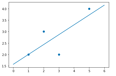
That seems fine, I mean there can be infinite lines but the one that best fits the given dataset is this one. And that’s what linear regression does it takes some set of input and linearly maps it to the output. Cool! So how do we find this line? Let’s see.
Working on Linear Regression
So in the above dataset, we have 2 variables x and y. So the equation of line we need to find is of form
y = m*x + c, but we’ll write it as:-

θo and θ1 are the same as c and m we’ll call them parameters. Our job is to find the value of parameters such that our hypothesis, hθ(x), minimizes the RMSE value. RMSE is called Root Mean Squared Error and it’s calculated by the following formula:-

Now we have 2 ways to go about it:-
- Gradient Descent
- Ordinary Least Square
Now, since in sklearn Linear Regression is done by OLS I’ll explain that since I’ll talk about Gradient Descent in the next article. For the above hypothesis we can find the parameters with the following formula:-

Now let’s try doing OLS on the above dataset:-
n = len(X)
theta_1 = ((n * (X*Y).sum()) - (X.sum() * Y.sum())) / ((n * (X**2).sum()) - X.sum()**2)
theta_0 = (Y.sum() - theta_1 * X.sum()) / n
print(theta_1, theta_0)

Well, the values look the same as we expected. But one thing to understand is that the above formula works only for data set where we have only one feature column. But in the real world that rarely happens so what about n feature columns?
Now we have a dataset with 2 features. Now let’s call this the X matrix now we have an X matrix with a shape (4,2) and let another matrix θ matrix which looks like [[θ1, θo]] and has a shape (1,2). Now we can write the hypothesis as the matrix multiplication of θT, i.e. transpose of θ matrix, and X matrix like:-

xo is still the column with all values as 1 and it can be rewritten as the matrix multiplication of θT and X.
Now that we know how it works let’s understand how we can code it.
Implementation of Linear Regression using sklearn
To implement Linear Regression we use a library called sklearn and it comes installed in Anaconda. Linear Regression is present in sklearn under linear_model. In this section, we will see how the Python Scikit-Learn library for machine learning can be used to implement regression functions. We will start with
simple linear regression involving two variables.
Loading the data
In this regression task, we will predict the percentage of marks that a student is expected to score based
on the number of hours they studied. You can download the data here. This is a simple linear regression task as it involves just two variables. So let’s start by importing the libraries and loading the data.
# Importing the required libraries
import pandas as pd
import numpy as np
import matplotlib.pyplot as plt
%matplotlib inline

# Loading the data
s_data = pd.read_csv("data.csv")
s_data.head()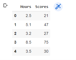
Let’s plot our data points on the 2D graph to eyeball our dataset and see if we can manually find any
relationship between the data. We can create the plot with the following lines of code
# Plotting the distribution of scores in a graph
s_data.plot(x='Hours', y='Scores', style='o')
plt.title('Hours vs Percentage')
plt.xlabel('Hours Studied')
plt.ylabel('Percentage Score')
plt.show()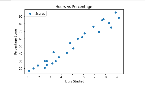
Linear Regression model
Now that we have our data let’s create our LinearRegression object and train it on the data. To train the data we use the fit() method. Let’s do it.
from sklearn.linear_model import LinearRegression

reg = LinearRegression()
reg.fit(X,Y)
From the graph above, we can clearly see that there is a positive linear relationship between the number of hours studied and percentage of the score.
Splitting the data
The next step is to divide the data into “attributes” (inputs) and “labels” (outputs). Now that we have our attributes and labels, the next step is to split this data into training and test sets. We’ll do this by using Scikit-Learn’s built-in train_test_split() method:
X = s_data.iloc[:, :-1].values
y = s_data.iloc[:, 1].values

from sklearn.model_selection import train_test_split
X_train, X_test, y_train, y_test = train_test_split(X, y,
                            test_size=0.2, random_state=0)
Training the model
We have split our data into training and testing sets, and now is finally the time to train our algorithm.
from sklearn.linear_model import LinearRegression
regressor = LinearRegression()
regressor.fit(X_train, y_train)

# Plotting the regression line
line = regressor.coef_*X+regressor.intercept_

# Plotting for the test data
plt.scatter(X, y)
plt.plot(X, line);
plt.show()

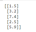
Now that we have trained our algorithm, it’s time to make some predictions.
# Testing the data
print(X_test)
Predicting the outcome
# Predicting the scores
y_pred = regressor.predict(X_test)

# Comparing Actual vs Predicted
df = pd.DataFrame({'Actual': y_test, 'Predicted': y_pred})
df 
# You can also test with your own data
hour = [[9.25]]
own_pred = regressor.predict(hour)
print("No of Hours = {}".format(hour))
print("Predicted Score = {}".format(own_pred[0]))
Evaluating the results
The final step is to evaluate the performance of the algorithm. This step is particularly important to compare how well different algorithms perform on a particular dataset. For simplicity here, we have chosen the mean square error. There are many such metrics.
# Calculating the mean absolute error
from sklearn import metrics
print('Mean Absolute Error:',
metrics.mean_absolute_error(y_test, y_pred)) 
Congrats! You just coded your first ML model. It’s not the best result but we’ll learn more as we go on.
Advantages of Linear Regression
- The implementation of Linear regression is very simple.
- Linear regression fits linearly separable datasets almost perfectly and is often used to find the nature of the relationship between variables.
- In Linear regression, the Overfitting of data can be reduced by regularization
Disadvantages of Linear Regression
- The linear regression algorithm is prone to underfitting
- It is sensitive to outliers
- The linear Regression algorithm assumes that the data is independent
Credits to edureka!
Thank for reading
Keep Learning
Tell us if you have any queries or if you found something wrong in this article.
Also Read:
- Machine Learning: A Gentle IntroductionIntroduction to Machine Learning Machine Learning is probably one of the most interesting and hyped branches of computer science. The thing that separates humans from machines is the fact that humans learn from their experiences. But is it possible to make a machine learn? And The answer is Yes! It is possible through Machine Learning….
- Machine Learning Course DescriptionBefore you start, let me give you an overview of what this series has to offer you. Our machine learning course series comprises of the following sections:- ML Environment Setup and Overview Jupyter Notebook: The Ultimate Guide Numpy Pandas Matplotlib Seaborn Sklearn Linear Regression Logistic Regression Decision Tree Random Forest Support Vector Machine K Nearest…
- ML Environment Setup and OverviewIntroduction to Machine Learning In this article, you will learn about the ML Environment Setup, Machine Learning terminology, its paradigms, and a tutorial to help you set up your machine so you can code what you learn. Before we start with our ML Environment Setup, read this article to get an overview of machine learning….
- Jupyter Notebook: The Ultimate GuideIntroduction to Jupyter Notebook Whenever one starts programming the first aim of that person is to find an IDE that suits his/her needs. In ML there are times when you’ll want to keep a check on your data after doing a change. But in code editors like Vim, Vscode, etc. you have to run your…
- Numpy For Machine Learning: A Complete GuideUp until now you’ve learned about the general idea of what ML does, set up your environment, and got to know about the working of your coding environment i.e. Jupyter Notebook. In this section, you’ll learn about a very powerful library called Numpy. We’ll learn about Numpy Array(np array for short) and operations on them,…
- Python Pandas Tutorial: A Complete Introduction for BeginnersIn the previous section, we learned about Numpy and how we can use it to load, save, and pre-process data easily by using Numpy Arrays. Now Numpy is a great library to do data preprocessing but I’d like to tell you all about another wonderful Python library called Pandas. At the end of this tutorial,…
- Matplotlib Python: A Beginner’s WalkthroughWe know how to analyze data by analyzing the statistics of the data and we’ve learned how to manipulate the data. But is statistics enough to analyze the data? Short answer, Visualization of data is necessary in order to find details that we missed that’s why Matplotlib Python is the best library to visualize data…
- Seaborn: Create Elegant PlotsIn the previous tutorial, we learned why data visualization is important and how we can create plots using matplotlib. In this tutorial, we’ll learn about another data visualization library called Seaborn, which is built on top of matplotlib. But why do we need seaborn if we have matplotlib? Using seaborn you can make plots that…
- Set up Python EnvironmentNow, it’s time to install the tools that we will use to write programs. So, we will be learning to Set up Python Environment in this article. Let’s start. 1. Installing Python first. First, we need to go to the official site of python: https://www.python.org/ Now we need to go to the downloads page of…
- Linear Regression: Your 1st Step in Machine LearningHi guys! So until now, we’ve learned about how we can use libraries to play with data. We did data analysis on a real dataset and we also learned how to visualize data. But what was the purpose behind it? Why do so many things? What are we trying to achieve? I’ll tell you all…
- Gradient Descent: Another Approach to Linear RegressionIn the last tutorial, we learned about our first ML algorithm called Linear Regression. We did it using an approach called Ordinary Least Squares, but there is another way to approach it. It is an approach that becomes the basis of Neural Networks, and it’s called Gradient Descent. And don’t get intimidated by the name…
- Logistic Regression: Regression Model for ClassificationWe will discuss Logistic Regression: Regression Model for Classification in this article, but let us see what we did in the past couple of articles, we discussed how we can use an ML algorithm called Linear Regression to predict continuous values by training it over a training dataset. We talked about 2 ways to do…
