Until now we already have a pretty good grasp of how things work when it comes to regression and classification. Today let’s take a ride back and learn about one of the first ML algorithms i.e. KNN or K Nearest Neighbours. The idea behind the algorithm is pretty straightforward. But it’s not something to be underestimated but something to look forward to. In the end, I also have an interesting use case of KNN. Let’s see if you can guess what it is. If you haven’t already, check out the pandas tutorial on our website.
K Nearest Neighbours Intuition
As I said KNN is a very straightforward algorithm. It’s actually the only algorithm that has O(1) train complexity and no training process. What! That doesn’t make sense though if it doesn’t train how does it know what to predict? That’s an absolutely valid question after all from all we have studied we train our model w.r.t. our dataset. If we don’t train them how can we derive proper inference? The answer lies in the technique that KNN uses to predict the outcome. Yes, it has no training process but that means it has a longer predicting process too. Let’s understand it with an example.
Example of KNN Algorithm
Let’s say we have a friend named Garry who wants to buy a house in a colony. The thing is Garry has a habit of agreeing to the initial price no matter how high and the broker knows this and tries to take advantage of the situation. You came to know about this and asked Garry to let you do the bidding instead. The thing you noticed is that the whole area has a pattern i.e. the houses near each other have similar prices. Knowing this you came up with a way to place to bid the correct price.

You three searched for a while and by the end of the day, Garry found the house he liked a lot. The Broker told the price to settle for and being greedy he said a price of $50k which was quite far-fetched. You denied the claims of the house being so pricey, Broker looked angry and asked how much do you think it is. You knew the price of 3 nearby houses i.e. $20k, $30k, and $25k. So you offered the average price of those i.e. 25k. The broker looked shocked and apologized for tricking Garry. Garry thanked you and treated you to a nice restaurant for the help.
Working of K Nearest Neighbours
The above example is pretty similar to the working of KNN. What KNN does is that it finds the points in the training set near to the point you want to predict the target for and gives you the majority class or average values of targets of those points depending on the type of problem you are solving i.e. Classification or Regression. But where does the k comes into play? More importantly what it is?
Previously I said KNN finds points nearby to the one we want to predict but how many points do we find the majority or average for? k is the no. of nearest points to consider for inference. For example, if k = 5 that means that we’ll take the nearest 5 points to infer the values from. The name makes sense since it takes k nearest points into consideration to infer the value.
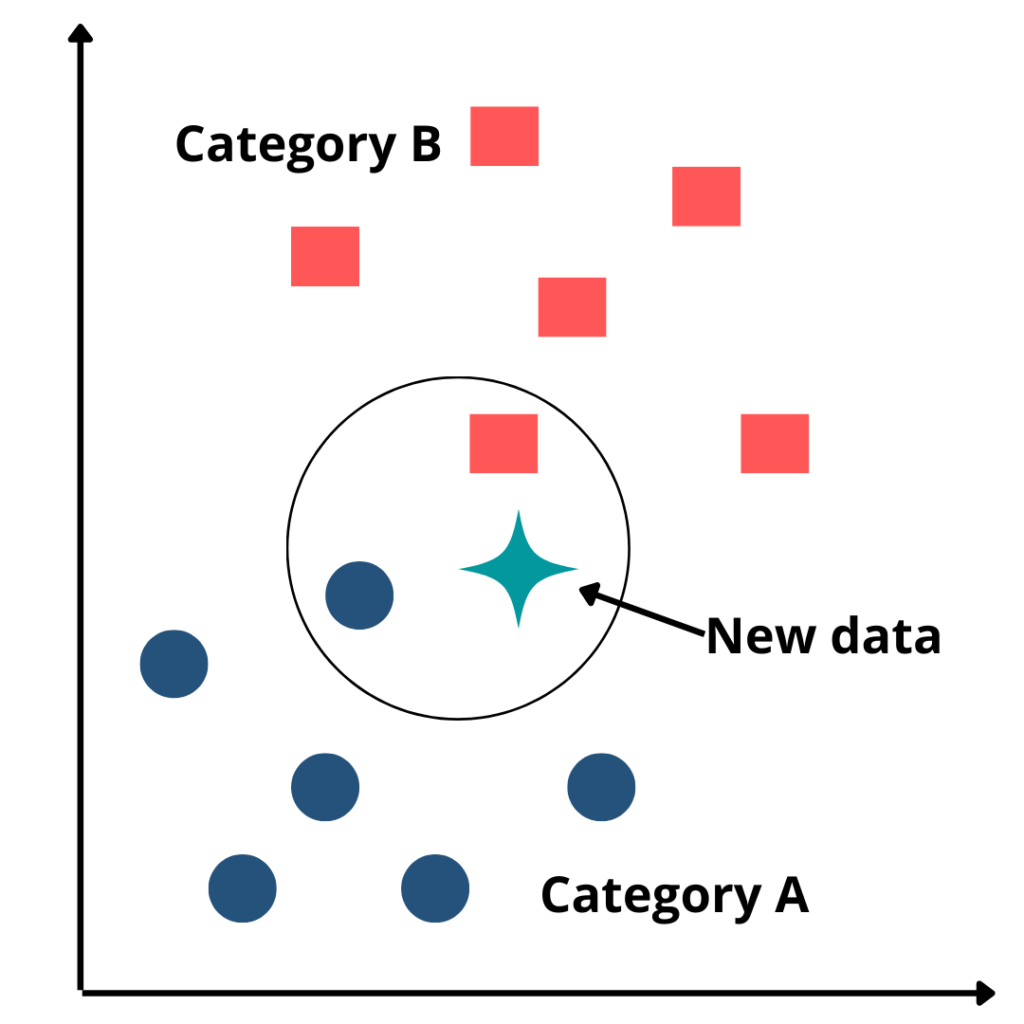
So how does this k affect the inference? The lower the value of k the more it is prone to overfit. The higher the value of k the more it is prone to be affected by outliers. Thus it is important to find the optimal value of k. Let’s see how we can do that.
Steps to build the K-NN algorithm
The K-NN working can be built on the basis of the below algorithm
Step-1: Select the number K of the neighbors. There is no particular way to determine the best value for “K”, so we need to try some values to find the best out of them. The most preferred value for K is 5. A very low value for K such as K=1 or K=2, can be noisy and lead to the effects of outliers in the model. Large values for K are good, but it may find some difficulties.
Step-2: Next, Calculate the Euclidean distance between the data points. The Euclidean distance is the distance between two points, which we have already studied in geometry.

Step-3: Take the K nearest neighbors as per the calculated Euclidean distance. Some ways to find optimal k value are
- Square Root Method: Take k as the square root of no. of training points. k is usually taken as odd no. so if it comes even using this, make it odd by +/- 1.
- Hyperparameter Tuning: Applying hyperparameter tuning to find the best value of k.
- Schwarz Criterion: The fanciest and over-the-top thing you can do. This works by minimizing distortion + λDklogN. Let’s not talk about it ever again!
Step-4: Among these k neighbors, count the number of the data points in each category. KNN assumes that similar points are closer to each other.
Step-5: After that, let’s assign the new data points to that category for which the number of the neighbor is maximum. It groups to the category which is near the data point.
Step-6: And that’s it, our KNN model is ready.
Implementation of KNN using sklearn
This was the surprise I was talking about and congrats if you guessed it correctly. For previous tutorials, the walkthroughs were getting a bit monotonous so I thought to spice things up a bit. So let’s get started with this tutorial we’ll recognize faces in the dataset Olivetti faces present in sklearn’s dataset. Let’s start with importing the required libraries and then importing our data.
#Importing the required libraries
import numpy as np
from sklearn.datasets import fetch_olivetti_faces
from sklearn.metrics import accuracy_score

#Importing the data
data = fetch_olivetti_faces()
X = data.data
Y = data.target
Now that we have our data let’s split it but one thing we see is that there are 40 different faces with 10 images of each face so when we split we want all the images in both sets. One way to make sure of that is to use stratify parameter which ensures the ratio of target classes is the same in the splits.
#Splitting the data into train and test data
from sklearn.model_selection import train_test_split
X_train, X_test, Y_train, Y_test = train_test_split(X, Y, stratify = Y)
Let’s train our model
#Import knearest neighbors Classifier model
from sklearn.neighbors import KNeighborsClassifier

#Training the model
clf = KNeighborsClassifier(n_neighbors=3)

#Train the model using the training sets
clf.fit(X_train, Y_train)

#Predict the response for test dataset
Y_pred = clf.predict(X_test)
Let’s find the accuracy which in this case came out to be 0.86.
#Import scikit-learn metrics module for accuracy calculation
from sklearn import metrics

# Calculating the Model Accuracy
print("Accuracy:",metrics.accuracy_score(Y_test, Y_pred))
Yay! You created a face recognition model with such ease and celebration. Also, KNN is pretty well suited for it given same faces are bound to have similar points making them cluster together near each other.
Advantages of K Nearest Neighbours
- No Training Period: It does not learn anything in the training period. It does not derive any discriminative function from the training data.
- Data can be updated easily and will not impact the accuracy of the algorithm.
- KNN algorithm is easy to implement
Disadvantages of K Nearest Neighbours
- Normalizing data is important else it could potentially lead to bad predictions.
- This algorithm doesn’t work well with large datasets.
- It doesn’t work well with high-dimension datasets.
Conclusion
Hope you have enjoyed this article about the KNN algorithm. We have looked into the KNN algorithm and its implementation in this article. Will meet you in the next article with an exciting new topic!
Credits: Edureka!
Also Read:
